Convolutional Neural Networks (CNNs)
ML models are trained on observed data to make decisions. Supervised learning, a subset of ML, maps input data to output predictions for regression or classification problems (Prince 2024). These types of models require labeled datasets comprised of input/output pairs to select the parameters of the mathematical equations underlying the models that best describe the data (Murphy 2022).
A Convolutional Neural Network (CNN) is a type of supervised learning model that contains convolutional layers, which are components of the model where the underlying mathematical operation is convolution (Prince 2024). For an image input, the convolution operation divides the image into overlapping 2D patches, then compares each patch with a set of small weight matrices, or “filters”. This comparison highlights features of the image that match the patterns stored in the filters. In this way, the convolution of the input image and the filters produce a feature map that can be passed into the next section of the model. The convolutional operation is also translationally invariant, so the model can detect whether a pattern is present anywhere in the input area rather than relying on a feature’s position within an input (Murphy 2022). This property is essential for image classification applications as a CNN should be able to identify an object regardless of its position.
The ifcbUTOPIA CNN, developed using the Keras library in Python and trained on labelled data from the NAAMES cruise, takes in pre-processed IFCB images and outputs a set of probabilities corresponding to 10 predetermined groups. The simplest Keras CNNs are comprised of a series of “Layers,” computation functions with stored weights that take in a tensor and output a transformed tensor. In these models, the output of one layer is input into the next. Key layers in the Keras library include:
- Input: Takes in the input data, which in our case is a preprocessed IFCB image, and instantiates a Keras tensor that can be propagated through the successive layers (Keras 2024).
- Convolution: Keras has several convolutional layers in its repertoire, including the “Conv2D” layer, which we used in our CNN. This layer type convolves the input tensor with the layer’s weight matrix over two dimensions, producing an output tensor (Keras 2024). 2D convolution compares input data to a set of small weight matrices called “filters.” This process highlights features that match the filter patterns, and the result of the convolution is a feature map (Prince 2024). Keras’ Conv2D layer can be customized with inputs to define attributes like number of filters, kernel size, padding, and stride length. If the padding is defined to be applied evenly with the value “same” and the stride length remains the default (1,1), the output tensor size remains equal to the input size (Keras 2024).
- Activation: Applies one of Keras’ “activation functions” to the input tensor. All of our activation layers use the Rectified Linear Unit function (ReLU), which takes the maximum of 0 and the input tensor value across each element of the tensor. This layer does not change the shape of the tensor; it only ensures that all values in the tensor are positive (Keras 2024). The inclusion of activation functions in the CNN structure prevents saturation, enabling construction of deeper, more complex models (Prince 2024).
- Batch Normalization: Standardizes the tensor statistics and enables scalability by applying a normalization transformation to the input tensor, maintaining a mean close to 0 and a standard deviation close to 1. The Keras Batch Normalization layer applies different function values depending on whether the CNN is in training or being used post-training. During training, normalization is applied using the mean and standard deviation of the current data, but during post-training evaluation, the function uses a moving average of the means and standard deviations of the training data (Keras 2024).
- Pooling: Pooling layers reduce the dimensionality of the data, introducing location invariance (Prince 2024). Our CNN uses the Keras MaxPooling2D layer, which performs the maximum pooling operation on two-dimensional spatial data. This operation takes the maximum value over an input window with dimensions defined by the layer, shifts the window, and repeats until all the data has been downsampled (Keras 2024).
- Flatten: This layer flattens the input tensor, an action that is useful when transitioning between two-dimensional layers like Conv2D and MaxPooling2D to one-dimensional Dense layers.
- Dense: A fundamental building block of neural networks, this layer is densely connected, meaning that each input node of this layer is connected to every output node. The Dense layer performs matrix-vector multiplication by taking the dot product of the input tensor and a weights matrix, adding a bias vector to the result, and applying an activation function to the sum (Keras 2024).
- Dropout: Keras’ Dropout layer is only active during model training and randomly sets input values to 0 at a rate defined by the developer, a process that helps to prevent overfitting. Data points that are not dropped are scaled up such that the overall sum of the input tensor is unchanged (Keras 2024).
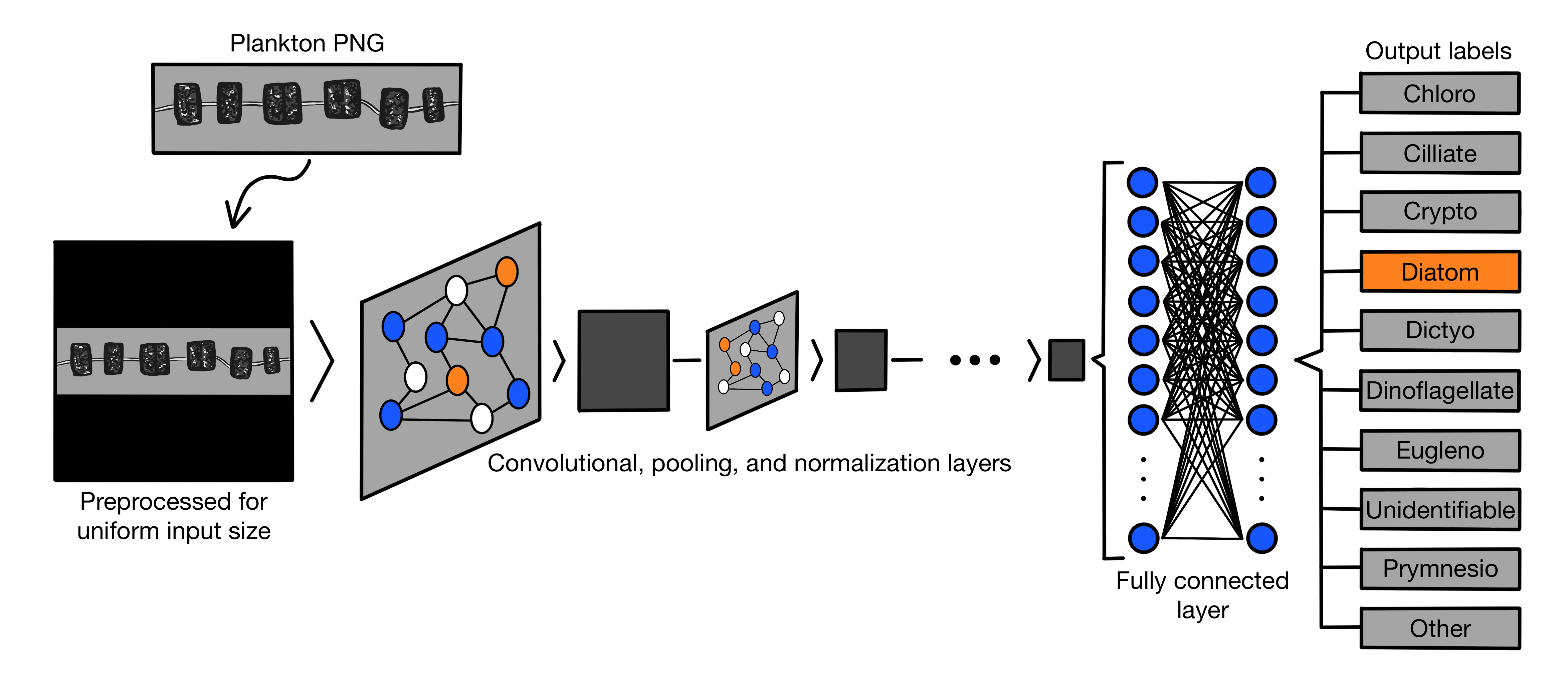
The ifcbUTOPIA CNN is constructed from 42 layers. To classify an image with the CNN, the image is entered as an input into the input layer, which then passes to a series of convolutional, activation, batch normalization, and pooling layers. The filter parameter of the convolutional layers is set to a new value with each pass, increasing or decreasing the complexity of the convolution function with the number of filters. Once convolution and pooling are complete, the data is flattened and passed to a dense layer, another set of activation and batch normalization layers, and a dropout layer before ending with another dense layer and a final ReLU activation layer. The output of the model is a set of 10 probabilities corresponding to the 10 classification groups. A visualization of the CNN structure is shown in the diagram above, and the code defining the model can be found in the ml-workflow repository.
Sources:
Keras. 2024. Keras 3 API Documentation. May 20. Accessed 2024. https://keras.io/api/.
LeCun, Yann, Yoshua Bengio, and Geoffrey Hinton. 2015. “Deep learning.” Nature 521: 436-444. https://www.nature.com/articles/nature14539.
Murphy, Kevin P. 2022. Probabilistic Machine Learning. Cambridge, MA: The MIT Press.
Prince, Simon J. D. 2024. Understanding Deep Learning. Cambridge, MA: The MIT Press.